pysheds
Simple and fast watershed delineation in Python.
https://github.com/mdbartos/pysheds
Category: Natural Resources
Sub Category: Water Supply and Quality
Keywords
accumulation catchments digital-elevation-model flow-direction gis hydrology
Keywords from Contributors
climate earth-system-model
Last synced: about 3 hours ago
JSON representation
Repository metadata
:earth_americas: Simple and fast watershed delineation in python.
- Host: GitHub
- URL: https://github.com/mdbartos/pysheds
- Owner: mdbartos
- License: gpl-3.0
- Created: 2017-04-13T16:02:37.000Z (almost 9 years ago)
- Default Branch: master
- Last Pushed: 2025-08-14T23:15:50.000Z (6 months ago)
- Last Synced: 2026-02-04T04:13:16.218Z (8 days ago)
- Topics: accumulation, catchments, digital-elevation-model, flow-direction, gis, hydrology
- Language: Python
- Homepage:
- Size: 14.5 MB
- Stars: 849
- Watchers: 29
- Forks: 226
- Open Issues: 94
- Releases: 9
-
Metadata Files:
- Readme: README.md
- License: LICENSE
README.md
pysheds 


🌎 Simple and fast watershed delineation in python.
Documentation
Read the docs here 📖.
Media
Hatari Labs - Elevation model conditioning and stream network delineation with python and pysheds 🇬🇧
Hatari Labs - Watershed and stream network delineation with python and pysheds 🇬🇧
Gidahatari - Delimitación de límite de cuenca y red hidrica con python y pysheds 🇪🇸
Earth Science Information Partners - Pysheds: a fast, open-source digital elevation model processing library 🇬🇧
Example usage
Example data used in this tutorial are linked below:
- Elevation: elevation.tiff
- Terrain: impervious_area.zip
- Soil Polygons: soils.zip
Additional DEM datasets are available via the USGS HydroSHEDS project.
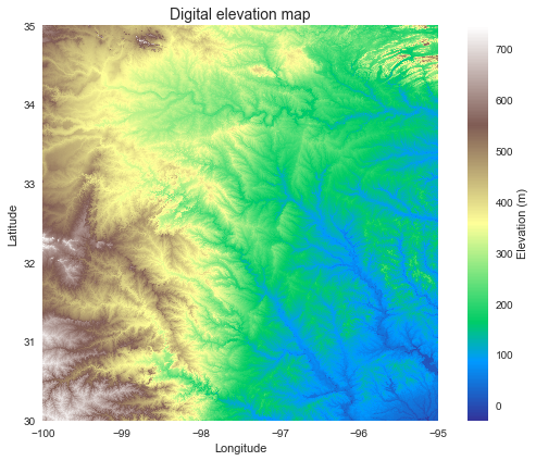
Read DEM data
# Read elevation raster
# ----------------------------
from pysheds.grid import Grid

grid = Grid.from_raster('elevation.tiff')
dem = grid.read_raster('elevation.tiff')
import numpy as np
import matplotlib.pyplot as plt
from matplotlib import colors
import seaborn as sns

fig, ax = plt.subplots(figsize=(8,6))
fig.patch.set_alpha(0)

plt.imshow(dem, extent=grid.extent, cmap='terrain', zorder=1)
plt.colorbar(label='Elevation (m)')
plt.grid(zorder=0)
plt.title('Digital elevation map', size=14)
plt.xlabel('Longitude')
plt.ylabel('Latitude')
plt.tight_layout()
Condition the elevation data
# Condition DEM
# ----------------------
# Fill pits in DEM
pit_filled_dem = grid.fill_pits(dem)

# Fill depressions in DEM
flooded_dem = grid.fill_depressions(pit_filled_dem)

# Resolve flats in DEM
inflated_dem = grid.resolve_flats(flooded_dem)
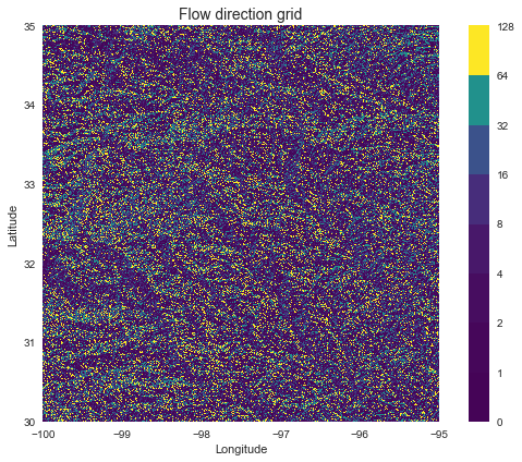
Elevation to flow direction
# Determine D8 flow directions from DEM
# ----------------------
# Specify directional mapping
dirmap = (64, 128, 1, 2, 4, 8, 16, 32)

# Compute flow directions
# -------------------------------------
fdir = grid.flowdir(inflated_dem, dirmap=dirmap)
fig = plt.figure(figsize=(8,6))
fig.patch.set_alpha(0)

plt.imshow(fdir, extent=grid.extent, cmap='viridis', zorder=2)
boundaries = ([0] + sorted(list(dirmap)))
plt.colorbar(boundaries= boundaries,
             values=sorted(dirmap))
plt.xlabel('Longitude')
plt.ylabel('Latitude')
plt.title('Flow direction grid', size=14)
plt.grid(zorder=-1)
plt.tight_layout()
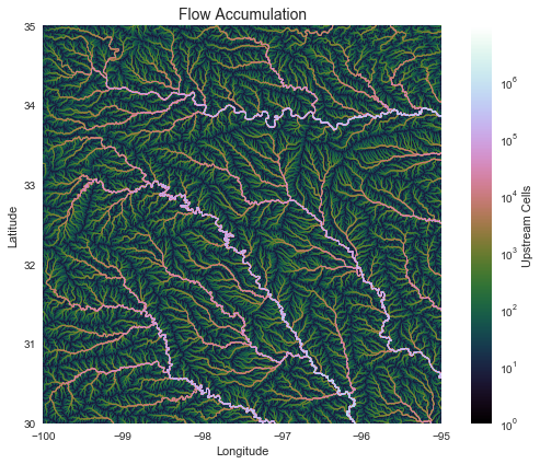
Compute accumulation from flow direction
# Calculate flow accumulation
# --------------------------
acc = grid.accumulation(fdir, dirmap=dirmap)
fig, ax = plt.subplots(figsize=(8,6))
fig.patch.set_alpha(0)
plt.grid('on', zorder=0)
im = ax.imshow(acc, extent=grid.extent, zorder=2,
               cmap='cubehelix',
               norm=colors.LogNorm(1, acc.max()),
               interpolation='bilinear')
plt.colorbar(im, ax=ax, label='Upstream Cells')
plt.title('Flow Accumulation', size=14)
plt.xlabel('Longitude')
plt.ylabel('Latitude')
plt.tight_layout()
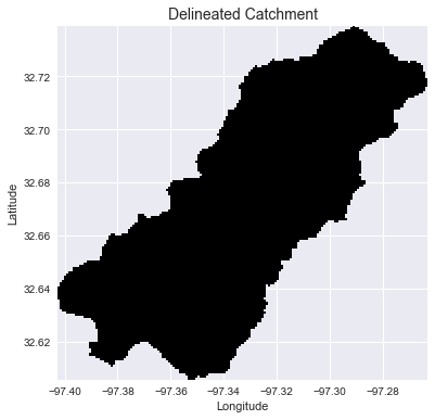
Delineate catchment from flow direction
# Delineate a catchment
# ---------------------
# Specify pour point
x, y = -97.294, 32.737

# Snap pour point to high accumulation cell
x_snap, y_snap = grid.snap_to_mask(acc > 1000, (x, y))

# Delineate the catchment
catch = grid.catchment(x=x_snap, y=y_snap, fdir=fdir, dirmap=dirmap,
                       xytype='coordinate')

# Crop and plot the catchment
# ---------------------------
# Clip the bounding box to the catchment
grid.clip_to(catch)
clipped_catch = grid.view(catch)
# Plot the catchment
fig, ax = plt.subplots(figsize=(8,6))
fig.patch.set_alpha(0)

plt.grid('on', zorder=0)
im = ax.imshow(np.where(clipped_catch, clipped_catch, np.nan), extent=grid.extent,
               zorder=1, cmap='Greys_r')
plt.xlabel('Longitude')
plt.ylabel('Latitude')
plt.title('Delineated Catchment', size=14)
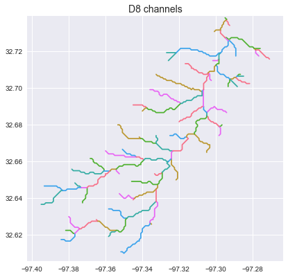
Extract the river network
# Extract river network
# ---------------------
branches = grid.extract_river_network(fdir, acc > 50, dirmap=dirmap)
sns.set_palette('husl')
fig, ax = plt.subplots(figsize=(8.5,6.5))

plt.xlim(grid.bbox[0], grid.bbox[2])
plt.ylim(grid.bbox[1], grid.bbox[3])
ax.set_aspect('equal')

for branch in branches['features']:
    line = np.asarray(branch['geometry']['coordinates'])
    plt.plot(line[:, 0], line[:, 1])

_ = plt.title('D8 channels', size=14)
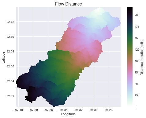
Compute flow distance from flow direction
# Calculate distance to outlet from each cell
# -------------------------------------------
dist = grid.distance_to_outlet(x=x_snap, y=y_snap, fdir=fdir, dirmap=dirmap,
                               xytype='coordinate')
fig, ax = plt.subplots(figsize=(8,6))
fig.patch.set_alpha(0)
plt.grid('on', zorder=0)
im = ax.imshow(dist, extent=grid.extent, zorder=2,
               cmap='cubehelix_r')
plt.colorbar(im, ax=ax, label='Distance to outlet (cells)')
plt.xlabel('Longitude')
plt.ylabel('Latitude')
plt.title('Flow Distance', size=14)
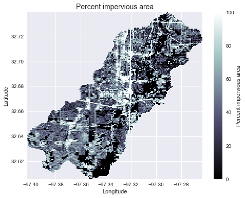
Add land cover data
# Combine with land cover data
# ---------------------
terrain = grid.read_raster('impervious_area.tiff', window=grid.bbox,
                           window_crs=grid.crs, nodata=0)
# Reproject data to grid's coordinate reference system
projected_terrain = terrain.to_crs(grid.crs)
# View data in catchment's spatial extent
catchment_terrain = grid.view(projected_terrain, nodata=np.nan)
fig, ax = plt.subplots(figsize=(8,6))
fig.patch.set_alpha(0)
plt.grid('on', zorder=0)
im = ax.imshow(catchment_terrain, extent=grid.extent, zorder=2,
               cmap='bone')
plt.colorbar(im, ax=ax, label='Percent impervious area')
plt.xlabel('Longitude')
plt.ylabel('Latitude')
plt.title('Percent impervious area', size=14)
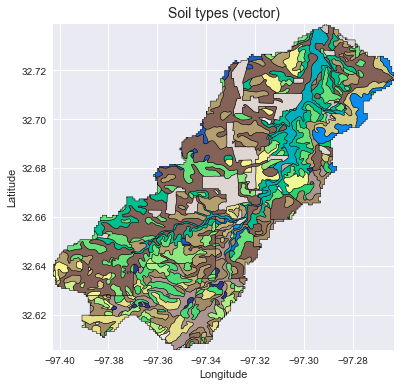
Add vector data
# Convert catchment raster to vector and combine with soils shapefile
# ---------------------
# Read soils shapefile
import pandas as pd
import geopandas as gpd
from shapely import geometry, ops
soils = gpd.read_file('soils.shp')
soil_id = 'MUKEY'
# Convert catchment raster to vector geometry and find intersection
shapes = grid.polygonize()
catchment_polygon = ops.unary_union([geometry.shape(shape)
                                     for shape, value in shapes])
soils = soils[soils.intersects(catchment_polygon)]
catchment_soils = gpd.GeoDataFrame(soils[soil_id],
                                   geometry=soils.intersection(catchment_polygon))
# Convert soil types to simple integer values
soil_types = np.unique(catchment_soils[soil_id])
soil_types = pd.Series(np.arange(soil_types.size), index=soil_types)
catchment_soils[soil_id] = catchment_soils[soil_id].map(soil_types)
fig, ax = plt.subplots(figsize=(8, 6))
catchment_soils.plot(ax=ax, column=soil_id, categorical=True, cmap='terrain',
                     linewidth=0.5, edgecolor='k', alpha=1, aspect='equal')
ax.set_xlim(grid.bbox[0], grid.bbox[2])
ax.set_ylim(grid.bbox[1], grid.bbox[3])
plt.xlabel('Longitude')
plt.ylabel('Latitude')
ax.set_title('Soil types (vector)', size=14)
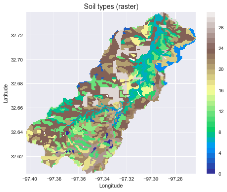
Convert from vector to raster
soil_polygons = zip(catchment_soils.geometry.values, catchment_soils[soil_id].values)
soil_raster = grid.rasterize(soil_polygons, fill=np.nan)
fig, ax = plt.subplots(figsize=(8, 6))
plt.imshow(soil_raster, cmap='terrain', extent=grid.extent, zorder=1)
boundaries = np.unique(soil_raster[~np.isnan(soil_raster)]).astype(int)
plt.colorbar(boundaries=boundaries,
             values=boundaries)
ax.set_xlim(grid.bbox[0], grid.bbox[2])
ax.set_ylim(grid.bbox[1], grid.bbox[3])
plt.xlabel('Longitude')
plt.ylabel('Latitude')
ax.set_title('Soil types (raster)', size=14)
Features
- Hydrologic Functions:
flowdir: Generate a flow direction grid from a given digital elevation dataset.catchment: Delineate the watershed for a given pour point (x, y).accumulation: Compute the number of cells upstream of each cell; if weights are
given, compute the sum of weighted cells upstream of each cell.distance_to_outlet: Compute the (weighted) distance from each cell to a given
pour point, moving downstream.distance_to_ridge: Compute the (weighted) distance from each cell to its originating
drainage divide, moving upstream.compute_hand: Compute the height above nearest drainage (HAND).stream_order: Compute the (strahler) stream order.extract_river_network: Extract river segments from a catchment and return a geojson
object.extract_profiles: Extract river segments and return a list of channel indices along with a dictionary describing connectivity.cell_dh: Compute the drop in elevation from each cell to its downstream neighbor.cell_distances: Compute the distance from each cell to its downstream neighbor.cell_slopes: Compute the slope between each cell and its downstream neighbor.fill_pits: Fill single-celled pits in a digital elevation dataset.fill_depressions: Fill multi-celled depressions in a digital elevation dataset.resolve_flats: Remove flats from a digital elevation dataset.detect_pits: Detect single-celled pits in a digital elevation dataset.detect_depressions: Detect multi-celled depressions in a digital elevation dataset.detect_flats: Detect flats in a digital elevation dataset.
- Viewing Functions:
view: Returns a "view" of a dataset defined by the grid's viewfinder.clip_to: Clip the viewfinder to the smallest area containing all non-
null gridcells for a provided dataset.nearest_cell: Returns the index (column, row) of the cell closest
to a given geographical coordinate (x, y).snap_to_mask: Snaps a set of points to the nearest nonzero cell in a boolean mask;
useful for finding pour points from an accumulation raster.
- I/O Functions:
read_ascii: Reads ascii gridded data.read_raster: Reads raster gridded data.from_ascii: Instantiates a grid from an ascii file.from_raster: Instantiates a grid from a raster file or Raster object.to_ascii: Write grids to delimited ascii files.to_raster: Write grids to raster files (e.g. geotiff).
pysheds supports both D8 and D-infinity routing schemes.
Installation
pysheds currently only supports Python 3.
Using pip
You can install pysheds using pip:
$ pip install pysheds
Using anaconda
First, add conda forge to your channels, if you have not already done so:
$ conda config --add channels conda-forge
Then, install pysheds:
$ conda install pysheds
Installing from source
For the bleeding-edge version, you can install pysheds from this github repository.
$ git clone https://github.com/mdbartos/pysheds.git
$ cd pysheds
$ python setup.py install
or
$ git clone https://github.com/mdbartos/pysheds.git
$ cd pysheds
$ pip install .
Performance
Performance benchmarks on a 2015 MacBook Pro (M: million, K: thousand):
| Function | Routing | Number of cells | Run time |
|---|---|---|---|
flowdir |
D8 | 36M | 1.14 [s] |
flowdir |
DINF | 36M | 7.01 [s] |
flowdir |
MFD | 36M | 4.21 [s] |
accumulation |
D8 | 36M | 3.44 [s] |
accumulation |
DINF | 36M | 14.9 [s] |
accumulation |
MFD | 36M | 32.5 [s] |
catchment |
D8 | 9.76M | 2.19 [s] |
catchment |
DINF | 9.76M | 3.5 [s] |
catchment |
MFD | 9.76M | 17.1 [s] |
distance_to_outlet |
D8 | 9.76M | 2.98 [s] |
distance_to_outlet |
DINF | 9.76M | 5.49 [s] |
distance_to_outlet |
MFD | 9.76M | 13.1 [s] |
distance_to_ridge |
D8 | 36M | 4.53 [s] |
distance_to_ridge |
DINF | 36M | 14.5 [s] |
distance_to_ridge |
MFD | 36M | 31.3 [s] |
hand |
D8 | 36M total, 730K channel | 12.3 [s] |
hand |
DINF | 36M total, 770K channel | 15.8 [s] |
hand |
MFD | 36M total, 770K channel | 29.8 [s] |
stream_order |
D8 | 36M total, 1M channel | 3.99 [s] |
extract_river_network |
D8 | 36M total, 345K channel | 4.07 [s] |
extract_profiles |
D8 | 36M total, 345K channel | 2.89 [s] |
detect_pits |
N/A | 36M | 1.80 [s] |
detect_flats |
N/A | 36M | 1.84 [s] |
fill_pits |
N/A | 36M | 2.52 [s] |
fill_depressions |
N/A | 36M | 27.1 [s] |
resolve_flats |
N/A | 36M | 9.56 [s] |
cell_dh |
D8 | 36M | 2.34 [s] |
cell_dh |
DINF | 36M | 4.92 [s] |
cell_dh |
MFD | 36M | 30.1 [s] |
cell_distances |
D8 | 36M | 1.11 [s] |
cell_distances |
DINF | 36M | 2.16 [s] |
cell_distances |
MFD | 36M | 26.8 [s] |
cell_slopes |
D8 | 36M | 4.01 [s] |
cell_slopes |
DINF | 36M | 10.2 [s] |
cell_slopes |
MFD | 36M | 58.7 [s] |
Speed tests were run on a conditioned DEM from the HYDROSHEDS DEM repository
(linked above as elevation.tiff).
Citing
If you have used this codebase in a publication and wish to cite it, consider citing the zenodo repository:
@misc{bartos_2020,
    title  = {pysheds: simple and fast watershed delineation in python},
    author = {Bartos, Matt},
    url    = {https://github.com/mdbartos/pysheds},
    year   = {2020},
    doi    = {10.5281/zenodo.3822494}
}
Owner metadata
- Name: Matt Bartos
- Login: mdbartos
- Email:
- Kind: user
- Description: Assistant Professor of Civil Engineering at UT Austin
- Website: future-water.github.io
- Location: Austin, TX
- Twitter:
- Company: @future-water, @ESIPFed
- Icon url: https://avatars.githubusercontent.com/u/8175317?u=b970ca0496ab3a237fa1346deb7762e0365835b3&v=4
- Repositories: 33
- Last ynced at: 2024-06-11T15:38:40.608Z
- Profile URL: https://github.com/mdbartos
GitHub Events
Total
- Pull request event: 8
- Fork event: 21
- Issues event: 11
- Watch event: 106
- Issue comment event: 35
- Push event: 3
- Create event: 1
Last Year
- Pull request event: 6
- Fork event: 15
- Issues event: 8
- Watch event: 67
- Issue comment event: 27
- Push event: 3
- Create event: 1
Committers metadata
Last synced: 9 days ago
Total Commits: 421
Total Committers: 10
Avg Commits per committer: 42.1
Development Distribution Score (DDS): 0.15
Commits in past year: 4
Committers in past year: 1
Avg Commits per committer in past year: 4.0
Development Distribution Score (DDS) in past year: 0.0
| Name | Commits | |
|---|---|---|
| Matt Bartos | m****s@u****u | 358 |
| Zeitsperre | 1****e | 16 |
| Ryan Grout | r****n@r****g | 14 |
| itati01 | i****1 | 13 |
| rickD | d****r@g****m | 8 |
| Philipp Kraft | p****t@u****e | 4 |
| Philipp Kraft | o****z@g****e | 3 |
| Matthew Plough | m****h@k****m | 2 |
| Jonathan King | j****3@g****m | 2 |
| David Huard | d****d@g****m | 1 |
Committer domains:
- koboldmetals.com: 1
- gmx.de: 1
- umwelt.uni-giessen.de: 1
- ryangrout.org: 1
- umich.edu: 1
Issue and Pull Request metadata
Last synced: 8 days ago
Total issues: 207
Total pull requests: 78
Average time to close issues: 10 months
Average time to close pull requests: 20 days
Total issue authors: 125
Total pull request authors: 20
Average comments per issue: 2.42
Average comments per pull request: 1.58
Merged pull request: 59
Bot issues: 0
Bot pull requests: 0
Past year issues: 12
Past year pull requests: 6
Past year average time to close issues: 5 days
Past year average time to close pull requests: 1 minute
Past year issue authors: 12
Past year pull request authors: 4
Past year average comments per issue: 2.33
Past year average comments per pull request: 0.33
Past year merged pull request: 0
Past year bot issues: 0
Past year bot pull requests: 0
Top Issue Authors
- mdbartos (39)
- itati01 (12)
- ShervanGharari (4)
- saikirankuntla (3)
- philippkraft (3)
- groutr (3)
- tommylees112 (3)
- JamesSample (3)
- hikmet34 (3)
- rishav-karanjit (3)
- fluviotect (3)
- DominiqueBrunet (2)
- Trevy05 (2)
- Omerhassanali (2)
- bhanu-magotra (2)
Top Pull Request Authors
- mdbartos (38)
- groutr (6)
- JonKing93 (5)
- itati01 (3)
- Zeitsperre (3)
- philippkraft (2)
- debboutr (2)
- JaweedNazary (2)
- alessandro-mariotti-zupit (2)
- ashleymedin (2)
- mplough-kobold (2)
- cheginit (2)
- Ledoux (2)
- feromes (1)
- avkoehl (1)
Top Issue Labels
- enhancement (12)
- bug (9)
- verify (1)
- help wanted (1)
- question (1)
Top Pull Request Labels
Package metadata
- Total packages: 1
- Total downloads: unknown
- Total dependent packages: 2
- Total dependent repositories: 2
- Total versions: 7
conda-forge.org: pysheds
Simple and fast watershed delineation in python.
- Homepage: https://github.com/mdbartos/pysheds
- Licenses: GPL-3.0-or-later
- Latest release: 0.3.3 (published over 3 years ago)
- Last Synced: 2026-02-03T12:11:56.735Z (8 days ago)
- Versions: 7
- Dependent Packages: 2
- Dependent Repositories: 2
-
Rankings:
- Forks count: 14.51%
- Stargazers count: 16.476%
- Average: 17.657%
- Dependent packages count: 19.581%
- Dependent repos count: 20.06%
Dependencies
- affine *
- geojson *
- numba *
- numpy *
- pandas *
- pyproj *
- rasterio >=1
- scikit-image *
- scipy *
- actions/checkout v2 composite
- actions/setup-python v2 composite
- actions/checkout v2 composite
- actions/setup-python v2 composite
- pypa/gh-action-pypi-publish 27b31702a0e7fc50959f5ad993c78deac1bdfc29 composite
Score: 10.537945736747394